Periodic Spline 1D [module]
Here are the methods of the class splinekit.PeriodicSpline1D.
This class handles periodic splines.
Properties
Constructors
Zero-Valued Spline
Periodized Spline Bases
From Data
Class Methods
Combine Two Splines
Evaluate Nonstandard Spline Representations
Instance Methods
Utility Methods
Evaluate a Spline
Empirical Statistics
Locations of Interest
Arithmetic and Geometric Operations
Calculus
Nonstandard Representations
Resampling and Projections
- class splinekit.periodic_spline_1d.PeriodicSpline1D
Bases:
objectThe class that maintains and operates on a polynomial one-dimensional uniform spline with periodic padding.
A uniform spline is a piecewise-polynomial function. The class
PeriodicSpline1Dis handling a version that is periodic, with the period \(K\in{\mathbb{N}}+1\) being a positive integer. The spline is\[f(x)=\sum_{k\in{\mathbb{Z}}}\,c[{k\bmod K}]\,\beta^{n}(x-\delta x-k),\]where \(x\in{\mathbb{R}}\) is the argument at which the spline \(f\) is evaluated, \(n\) is the nonnegative degree of the polynomial spline, \(\beta^{n}\) is a B-spline synthesis function, and \(\delta x\) is a delay that controls the placement of the uniform knots. The array of coefficients \(c\) is giving its shape to the spline.
- degree
(R/W) The nonnegative degree \(n\in{\mathbb{N}}\) of the polynomial spline.
- Type:
int
- delay
(R/W) The delay \(\delta x\in{\mathbb{R}}.\)
- Type:
float
- spline_coeff
(R/W) The spline coefficients \(c\in{\mathbb{R}}^{K}.\) The setter creates a local copy and updates the period.
- Type:
np.ndarray[tuple[int], np.dtype[np.float64]]
- Raises:
ValueError – Raised when
degreeis negative.ValueError – Raised when
spline_coefffails to be anumpyone-dimensionalfloatarray that contains at least one element.
- __init__() None
The default constructor for this class.
Creates a piecewise-constant periodic spline of unit period, vanishing delay, and value zero.
- Parameters:
None
Examples
- Load the library.
>>> import splinekit as sk
- Create a default spline.
>>> sk.PeriodicSpline1D()
PeriodicSpline1D([0.], degree = 0, delay = 0.0)
- classmethod periodized_b_spline(*, period: int, degree: int) PeriodicSpline1D
The constructor of a periodized B-spline.
This constructor populates the attributes of a
PeriodicSpline1Dobject that represents the one-dimensional spline\[f(x)=\sum_{k\in{\mathbb{Z}}}\,\beta^{n}(k\,K+x),\]as defined here. This spline has period \(K\) and is the periodized version of a centered B-spline of degree \(n.\)
- Parameters:
period (int) – The positive period of the periodized B-spline.
degree (int) – The nonnegative degree of the periodized B-spline.
- Returns:
The periodized B-spline centered at the origin.
- Return type:
Examples
- Load the library.
>>> import splinekit as sk
- Create a nonic B-spline of period
6. >>> sk.PeriodicSpline1D.periodized_b_spline(period = 6, degree = 9) PeriodicSpline1D([1. 0. 0. 0. 0. 0.], degree = 9, delay = 0.0)
- Raises:
ValueError – Raised when
periodis nonpositive.ValueError – Raised when
degreeis negative.
- classmethod periodized_cardinal_b_spline(*, period: int, degree: int) PeriodicSpline1D
The constructor of a periodized cardinal B-spline.
This constructor populates the attributes of a
PeriodicSpline1Dobject that represents the one-dimensional spline\[f(x)=\sum_{k\in{\mathbb{Z}}}\,\eta^{n}(k\,K+x),\]as defined here. This spline has period \(K\) and is the periodized version of a centered cardinal B-spline of degree \(n.\)
- Parameters:
period (int) – The positive period of the periodized cardinal B-spline.
degree (int) – The nonnegative degree of the periodized cardinal B-spline.
- Returns:
The periodized cardinal B-spline centered at the origin.
- Return type:
Examples
- Load the library.
>>> import splinekit as sk
- Create a nonic cardinal B-spline of period
6. >>> sk.PeriodicSpline1D.periodized_cardinal_b_spline(period = 6, degree = 9) PeriodicSpline1D([10.54181435 -8.30274513 6.41054444 -5.75741296 6.41054444 -8.30274513], degree = 9, delay = 0.0)
- Raises:
ValueError – Raised when
periodis nonpositive.ValueError – Raised when
degreeis negative.
- classmethod periodized_dual_b_spline(*, period: int, dual_degree: int, primal_degree: int) PeriodicSpline1D
The constructor of a periodized dual B-spline.
This constructor populates the attributes of a
PeriodicSpline1Dobject that represents the one-dimensional spline\[f(x)=\sum_{k\in{\mathbb{Z}}}\,\mathring{\beta}^{m,n}(k\,K+x),\]as defined here. This spline has period \(K\) and is the periodized version of a centered dual B-spline of dual degree \(m\) and primal degree \(n.\)
- Parameters:
period (int) – The positive period of the periodized dual B-spline.
dual_degree (int) – The nonnegative dual degree of the periodized dual B-spline.
primal_degree (int) – The nonnegative primal degree of the periodized dual B-spline.
- Returns:
The periodized dual B-spline centered at the origin.
- Return type:
Examples
- Load the library.
>>> import splinekit as sk
- Create a nonic dual B-spline of quadratic primal degree and period
6. >>> sk.PeriodicSpline1D.periodized_dual_b_spline(period = 6, dual_degree = 9, primal_degree = 2) PeriodicSpline1D([ 34.24972088 -31.03664923 27.43176629 -26.039955 27.43176629 -31.03664923], degree = 9, delay = 0.0)
- Raises:
ValueError – Raised when
periodis nonpositive.ValueError – Raised when
dual_degreeis negative.ValueError – Raised when
primal_degreeis negative.
- classmethod periodized_orthonormal_b_spline(*, period: int, degree: int) PeriodicSpline1D
The constructor of a periodized orthonormal B-spline.
This constructor populates the attributes of a
PeriodicSpline1Dobject that represents the one-dimensional spline\[f(x)=\sum_{k\in{\mathbb{Z}}}\,\phi^{n}(k\,K+x),\]as defined here. This spline has period \(K\) and is the periodized version of a centered orthonormal B-spline of degree \(n.\)
- Parameters:
period (int) – The positive period of the periodized orthonormal B-spline.
degree (int) – The nonnegative degree of the periodized orthonormal B-spline.
- Returns:
The periodized orthonormal B-spline centered at the origin.
- Return type:
Examples
- Load the library.
>>> import splinekit as sk
- Create a nonic orthonormal B-spline of period
6. >>> sk.PeriodicSpline1D.periodized_orthonormal_b_spline(period = 6, degree = 9) PeriodicSpline1D([ 13.70088094 -11.4607243 9.56634894 -8.91213021 9.56634894 -11.4607243 ], degree = 9, delay = 0.0)
- Raises:
ValueError – Raised when
periodis nonpositive.ValueError – Raised when
degreeis negative.
- classmethod from_samples(samples: ndarray[tuple[int], dtype[float64]], *, degree: int, delay: float = 0.0, regularized: bool = False) PeriodicSpline1D
A constructor from data samples.
This constructor populates the attributes of a
PeriodicSpline1Dobject, which represents the one-dimensional spline\[f(x)=\sum_{k\in{\mathbb{Z}}}\,c[{k\bmod K}]\, \beta^{n}(x-\delta x-k),\]as defined here. The provided data samples \(\left(s[k]\right)_{k=0}^{K-1}\) are assumed to have been taken at the integers.
When
regularized == False, this constructor determines the spline coefficients \(\left(c[k]\right)_{k=0}^{K-1}\) such that the periodic spline \(f\) interpolates the samples \(s,\) meaning that \(\left(f(k)\right)_{k=0}^{K-1}= \left(s[k]\right)_{k=0}^{K-1}.\) In general, this condition can be satisfied for any delay \(\delta x\in{\mathbb{R}},\) provided the period \(K\in2\,{\mathbb{N}}+1\) is odd. Alternatively, the interpolation condition can be satisfied for any non-half-integer delay \(\delta x\in{\mathbb{R}}\setminus \left({\mathbb{Z}}+\frac{1}{2}\right),\) this time without restriction on the parity of the positive period \(K\in{\mathbb{N}}+1.\)For an even period \(K\in2\,{\mathbb{N}}+2\) combined with a half-integer delay \(\delta x\in{\mathbb{Z}}+\frac{1}{2},\) the directive
regularized == Falseis disregraded and regularization is enforced.When
regularized == True, the interpolation condition is still honored for all odd periods. For even periods \(K\in2\,{\mathbb{N}}+2,\) however, this constructor determines the spline coefficients \(\left(c[k]\right)_{k=0}^{K-1}\) that minimize the criterion \(J=\sum_{k=0}^{K-1}\,\left(f(k)-s[k]\right)^{2}\) such that \(\sum_{k=0}^{K/2-1}\,f(2\,k)=\sum_{k=0}^{K/2-1}\,f(2\,k+1),\) which happens to lift the restriction of non-half-integer delays.
- Parameters:
samples (np.ndarray[tuple[int], np.dtype[np.float64]]) – A one-dimensional
numpyarray of real data samples. The period of the spline will be set to the length of this array.degree (int) – The nonnegative degree of the polynomial spline.
delay (float) – The delay of this spline.
regularized (bool) – The regularization directive.
- Returns:
The spline.
- Return type:
Examples
- Load the libraries.
>>> import numpy as np
>>> import splinekit as sk
- Create a spline from a few samples.
>>> samples = np.array([1, 5, -3], dtype = float)
>>> sk.PeriodicSpline1D.from_samples(samples, degree = 3)
PeriodicSpline1D([ 1.  9. -7.], degree = 3, delay = 0.0)
- Raises:
ValueError – Raised when
samplesfails to be anumpyone-dimensionalfloatarray that contains at least one element.ValueError – Raised when
degreeis negative.
- classmethod from_smoothed_samples(samples: ndarray[tuple[int], dtype[float64]], *, degree: int, delay: float = 0.0, smoothing: ndarray[tuple[int], dtype[float64]]) PeriodicSpline1D
A constructor from data samples.
This constructor populates the attributes of a
PeriodicSpline1Dobject, which represents the one-dimensional spline\[f(x)=\sum_{k\in{\mathbb{Z}}}\,c[{k\bmod K}]\, \beta^{n}(x-\delta x-k),\]as defined here. The provided data samples \(\left(s[k]\right)_{k=0}^{K-1}\) are assumed to have been taken at the integers.
The constructed spline minimizes the criterion
\[J=\sum_{k=0}^{K-1}\,\left(f(k)-s[k]\right)^{2}+\sum_{m=0}^{n}\, \lambda[m]\,\int_{0}^{K}\, \left(\frac{{\mathrm{d}}^{m}f(x)}{{\mathrm{d}}x^{m}}\right)^{2}\, {\mathrm{d}}x.\]The first term encourages the spline to interpolate the samples, while the second term discourages the spline derivatives to be large, as controlled by the vector \(\left(\lambda[m]\right)_{m=0}^{n}\) of smoothing parameters.
- Parameters:
samples (np.ndarray[tuple[int], np.dtype[np.float64]]) – A one-dimensional
numpyarray of real data samples. The period of the spline will be set to the length of this array.degree (int) – The nonnegative degree of the polynomial spline.
delay (float) – The delay of this spline.
smoothing (np.ndarray[tuple[int], np.dtype[np.float64]]) – A one-dimensional
numpyarray ofn + 1regularization weights.
- Returns:
The spline.
- Return type:
Examples
- Load the libraries.
>>> import numpy as np
>>> import splinekit as sk
- Create a cubic spline with highly attenuated second-order derivatives.
>>> samples = np.array([1, 5, -3], dtype = float)
>>> regularization = np.array([0, 0, 5, 0], dtype = float)
>>> sk.PeriodicSpline1D.from_smoothed_samples(samples, degree = 3, smoothing = regularization)
PeriodicSpline1D([1.         1.08791209 0.91208791], degree = 3, delay = 0.0)
- Raises:
ValueError – Raised when
samplesfails to be anumpyone-dimensionalfloatarray that contains at least one element.ValueError – Raised when
degreeis negative.ValueError – Raised when
smoothingfails to be anumpyone-dimensionalfloatarray that containsdegree + 1elements.
- classmethod from_spline_coeff(spline_coeff: ndarray[tuple[int], dtype[float64]], *, degree: int, delay: float = 0.0) PeriodicSpline1D
A constructor from spline coefficients.
This constructor populates the attributes of a
PeriodicSpline1Dobject with the provided parameters. The created object retains a copy of the arrayspline_coeff.- Parameters:
spline_coeff (np.ndarray[tuple[int], np.dtype[np.float64]]) – A one-dimensional
numpyarray of real spline coefficients. The period of the spline will be set to the length of this array.degree (int) – The nonnegative degree of the polynomial spline.
delay (float) – The delay of this spline.
- Returns:
The spline.
- Return type:
Examples
- Load the libraries.
>>> import numpy as np
>>> import splinekit as sk
- Create a spline from a few coefficients.
>>> c = np.array([1, 9, -7], dtype = float)
>>> sk.PeriodicSpline1D.from_spline_coeff(c, degree = 3)
PeriodicSpline1D([ 1.  9. -7.], degree = 3, delay = 0.0)
- Raises:
ValueError – Raised when
spline_coefffails to be anumpyone-dimensionalfloatarray that contains at least one element.ValueError – Raised when
degreeis negative.
- classmethod add(augend: PeriodicSpline1D, addend: PeriodicSpline1D) PeriodicSpline1D
Create a spline from the sum of two splines.
Given two
PeriodicSpline1Dobjects of identical period \(K,\) degree \(n,\) and delay \(\delta x,\) this constructor returns a newPeriodicSpline1Dspline that represents their sum. The created object has period \(K,\) degree \(n,\) and delay \(\delta x,\) too.- Parameters:
augend (PeriodicSpline1D) – A
PeriodicSpline1Dspline.addend (PeriodicSpline1D) – A
PeriodicSpline1Dspline.
- Returns:
The spline equal to the sum of
augendandaddend.- Return type:
Examples
- Load the libraries.
>>> import numpy as np
>>> import splinekit as sk
- Create two undelayed cubic splines and sum them.
>>> c1 = np.array([1, 9, -7], dtype = float)
>>> s1 = sk.PeriodicSpline1D.from_spline_coeff(c1, degree = 3)
>>> c2 = np.array([6, -3, -2], dtype = float)
>>> s2 = sk.PeriodicSpline1D.from_spline_coeff(c2, degree = 3)
>>> sk.PeriodicSpline1D.add(s1, s2)
PeriodicSpline1D([ 7.  6. -9.], degree = 3, delay = 0.0)
- Raises:
ValueError – Raised when
augend.period != addend.period.ValueError – Raised when
augend.degree != addend.degree.ValueError – Raised when
augend.delay != addend.delay.
- classmethod add_projected(augend: PeriodicSpline1D, addend: PeriodicSpline1D, *, degree: int, delay: float = 0.0) PeriodicSpline1D
Create a spline of arbitrary degree and delay from the sum of two splines.
Given two
PeriodicSpline1Dobjects of identical period \(K,\) independent degree \((n_{1}, n_{2}),\) and independent delay \((\delta x_{1}, \delta x_{2}),\) this constructor returns a newPeriodicSpline1Dspline that represents the continuous least-squares approximation of their sum by aPeriodicSpline1Dspline of period \(K,\) nonnegative degree \(n,\) and delay \(\delta x\in{\mathbb{R}}.\)With
\[\begin{split}\begin{array}{rcl} s_{1}(x)&=&\sum_{k\in{\mathbb{Z}}}\,c_{1}[{k\bmod K}]\, \beta^{n_{1}}(x-\delta x_{1}-k)\\ s_{2}(x)&=&\sum_{k\in{\mathbb{Z}}}\,c_{2}[{k\bmod K}]\, \beta^{n_{2}}(x-\delta x_{2}-k), \end{array}\end{split}\]the created sum
\[f(x)=\sum_{k\in{\mathbb{Z}}}\,c[{k\bmod K}]\, \beta^{n}(x-\delta x-k)\]minimizes the criterion \(J=\int_{0}^{K}\,\left(f(x)-s_{1}(x)- s_{2}(x)\right)^{2}\,{\mathrm{d}}x\) in terms of the coefficients \(c.\)
- Parameters:
augend (PeriodicSpline1D) – A
PeriodicSpline1Dspline.addend (PeriodicSpline1D) – A
PeriodicSpline1Dspline.degree (int) – The nonnegative degree of the created polynomial spline.
delay (float) – The delay of the created spline.
- Returns:
The spline of degree
degreeand delaydelaythat best approximates the sum ofaugendandaddend.- Return type:
Examples
- Load the libraries.
>>> import numpy as np
>>> import splinekit as sk
- Create two splines and sum them.
>>> c1 = np.array([1, 9, -7], dtype = float)
>>> s1 = sk.PeriodicSpline1D.from_spline_coeff(c1, degree = 3, delay = 8.4)
>>> c2 = np.array([6, -3, -2], dtype = float)
>>> s2 = sk.PeriodicSpline1D.from_spline_coeff(c2, degree = 1, delay = 0.1)
>>> sk.PeriodicSpline1D.add_projected(s1, s2, degree = 0, delay = -4.25)
PeriodicSpline1D([-4.72426875  6.28725     2.43701875], degree = 0, delay = -4.25)
- Raises:
ValueError – Raised when
augend.period != addend.period.ValueError – Raised when
degreeis negative.
- classmethod convolve(s1: PeriodicSpline1D, s2: PeriodicSpline1D) PeriodicSpline1D
Create a spline from the convolution of two splines.
Given two
PeriodicSpline1Dobjects of identical period \(K,\) independent degree \((n_{1}, n_{2}),\) and independent delay \((\delta x_{1}, \delta x_{2}),\) this constructor returns a newPeriodicSpline1Dspline that represents their convolution. The created object has period \(K,\) too.With
\[\begin{split}\begin{array}{rcl} s_{1}(x)&=&\sum_{k\in{\mathbb{Z}}}\,c_{1}[{k\bmod K}]\, \beta^{n_{1}}(x-\delta x_{1}-k)\\ s_{2}(x)&=&\sum_{k\in{\mathbb{Z}}}\,c_{2}[{k\bmod K}]\, \beta^{n_{2}}(x-\delta x_{2}-k), \end{array}\end{split}\]the created convolution result is
\[f(x)=\int_{0}^{K}\,s_{1}(y)\,s_{2}(x-y)\,{\mathrm{d}}y.\]- Parameters:
s1 (PeriodicSpline1D) – A
PeriodicSpline1Dspline.s2 (PeriodicSpline1D) – A
PeriodicSpline1Dspline.
- Returns:
The spline equal to the convolution of
s1ands2.- Return type:
Examples
- Load the libraries.
>>> import numpy as np
>>> import splinekit as sk
- Create two splines and convolve them.
>>> c1 = np.array([1, 9, -7], dtype = float)
>>> s1 = sk.PeriodicSpline1D.from_spline_coeff(c1, degree = 3, delay = 8.4)
>>> c2 = np.array([6, -3, -2], dtype = float)
>>> s2 = sk.PeriodicSpline1D.from_spline_coeff(c2, degree = 1, delay = 0.1)
>>> sk.PeriodicSpline1D.convolve(s1, s2)
PeriodicSpline1D([  9.  65. -71.], degree = 5, delay = 8.5)
- Raises:
ValueError – Raised when
s1.period != s2.period.
- classmethod normed_cross_correlate(s1: PeriodicSpline1D, s2: PeriodicSpline1D) PeriodicSpline1D
Create a spline from the normalized cross-correlation of two splines.
Given two
PeriodicSpline1Dobjects of identical period \(K,\) independent degree \((n_{1}, n_{2}),\) and independent delay \((\delta x_{1}, \delta x_{2}),\) this constructor returns a newPeriodicSpline1Dspline that represents their zero-normalized cross-correlation. The created object has period \(K,\) too.With
\[\begin{split}\begin{array}{rcl} s_{1}(x)&=&\sum_{k\in{\mathbb{Z}}}\,c_{1}[{k\bmod K}]\, \beta^{n_{1}}(x-\delta x_{1}-k)\\ s_{2}(x)&=&\sum_{k\in{\mathbb{Z}}}\,c_{2}[{k\bmod K}]\, \beta^{n_{2}}(x-\delta x_{2}-k), \end{array}\end{split}\]the created zero-normalized cross-correlation result \(f(x)\in[-1,1]\) is
\[f(x)=\frac{1}{K}\,\int_{0}^{K}\,\frac{s_{1}(y)- {\mathrm{E}}\{s_{1}\}}{\sqrt{{\mathrm{Var}}\{s_{1}\}}}\, \frac{s_{2}(y+x)}{\sqrt{{\mathrm{Var}}\{s_{2}\}}}\,{\mathrm{d}}y,\]where \({\mathrm{E}}\) is the mean value of a spline and \({\mathrm{Var}}\) is its variance.
- Parameters:
s1 (PeriodicSpline1D) – A
PeriodicSpline1Dspline.s2 (PeriodicSpline1D) – A
PeriodicSpline1Dspline.
- Returns:
The spline equal to the zero-normalized cross-correlation of
s1ands2.- Return type:
Examples
- Load the libraries.
>>> import numpy as np
>>> import splinekit as sk
- Create two splines and cross-correlate them.
>>> c1 = np.array([1, 9, -7], dtype = float)
>>> s1 = sk.PeriodicSpline1D.from_spline_coeff(c1, degree = 3, delay = 8.4)
>>> c2 = np.array([6, -3, -2], dtype = float)
>>> s2 = sk.PeriodicSpline1D.from_spline_coeff(c2, degree = 1, delay = 0.1)
>>> sk.PeriodicSpline1D.normed_cross_correlate(s1, s2)
PeriodicSpline1D([-0.30586209 -2.44689675  2.75275884], degree = 5, delay = -8.3)
- Raises:
ValueError – Raised when
s1.period != s2.period.ValueError – Raised when
0.0 == s1.variance().ValueError – Raised when
0.0 == s2.variance().
- classmethod eval_piecewise_polynomials_at(x: float, polynomials: PeriodicNonuniformPiecewise) float
The ordinate of a piecewise polynomial at an arbitrary abscissa.
Evaluated at the abscissa
x, this function returns the value of a given PeriodicNonuniformPiecewise object that represents a periodic piecewise polynomial, as made available by the function piecewise_polynomials.The evaluation proceeds in two steps. The first step is to identify which piece of the piecewise polynomial the abscissa belongs to. The second step is to evaluate the ordinate by direct computation of the polynomial.
- Parameters:
x (float) – The abscissa.
polynomials (PeriodicNonuniformPiecewise) – A piecewise-polynomial function.
- Returns:
The value of the piecewise polynomial evaluated at
x.- Return type:
float
Examples
- Load the libraries.
>>> import numpy as np
>>> import splinekit as sk
- Create a spline and evaluate it from its pievewise-polynomial representation.
>>> c = np.array([1, 9, -7], dtype = float)
>>> s = sk.PeriodicSpline1D.from_spline_coeff(c, degree = 3)
>>> pp = s.piecewise_polynomials()
>>> x = -18.5
>>> print(sk.PeriodicSpline1D.eval_piecewise_polynomials_at(x, pp))
>>> print(s.at(x))
>>> print(s.at(x) - sk.PeriodicSpline1D.eval_piecewise_polynomials_at(x, pp))
-2.499999999999999
-2.5
-8.881784197001252e-16
See also
atEvaluation of this spline at
x.
- classmethod eval_piecewise_sgn_at(x: float, sgn: PeriodicNonuniformPiecewise) float
The signum, at an arbitrary abscissa, of the PeriodicNonuniformPiecewise object returned by the function piecewise_sgn().
Evaluated at the abscissa
x, this function returns the value of a given PeriodicNonuniformPiecewise object that represents the signum of a periodic spline, as made available by the function piecewise_sgn.The evaluation proceeds in two steps. The first step is to identify which piece of the piecewise signum the abscissa belongs to. The second step is to evaluate the ordinate by direct lookup of the signum.
- Parameters:
x (float) – The abscissa.
sgn (PeriodicNonuniformPiecewise) – A piecewise-signum function.
- Returns:
The value of the piecewise signum evaluated at
x.- Return type:
float
Examples
- Load the libraries.
>>> import numpy as np
>>> import splinekit as sk
- Create a spline and evaluate it from its pievewise-signum representation.
>>> c = np.array([1, 9, -7], dtype = float)
>>> s = sk.PeriodicSpline1D.from_spline_coeff(c, degree = 3)
>>> ps = s.piecewise_sgn()
>>> x = -18.5
>>> print(sk.PeriodicSpline1D.eval_piecewise_sgn_at(x, ps))
>>> print(np.sign(s.at(x)))
-1.0
-1.0
See also
atEvaluation of this spline at
x.
- copy() PeriodicSpline1D
A copy of this object.
This function returns a deep copy of this object.
- Parameters:
None
- Returns:
The copied spline.
- Return type:
Examples
- Load the libraries.
>>> import numpy as np
>>> import splinekit as sk
- Create a spline and duplicate it.
>>> c = np.array([1, 9, -7], dtype = float)
>>> s1 = sk.PeriodicSpline1D.from_spline_coeff(c, degree = 3, delay = 8.4)
>>> s2 = s1.copy()
>>> s1
PeriodicSpline1D([ 1.  9. -7.], degree = 3, delay = 8.4)
>>> s2
PeriodicSpline1D([ 1.  9. -7.], degree = 3, delay = 8.4)
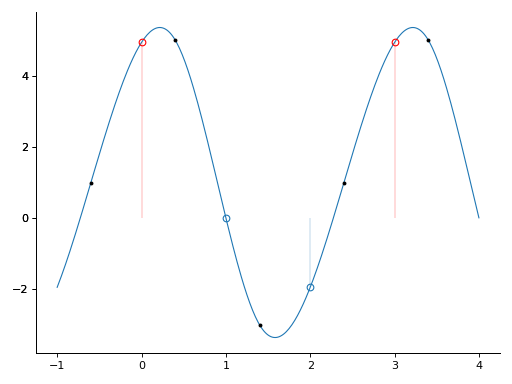
- plot(subplot: Tuple[plt.Figure, plt.Axes], *, plotdomain: Interval = RR(), plotrange: Interval = RR(), plotpoints: int, curve_fmt: str = '-C0', curve_lw: float = 1.0, curve_markerfmt: str = 'oC0', curvestem_linefmt: str = '-C0', knot_marker: str = 'o', knot_color: str = 'k', periodbound_markerfmt: str = 'or', periodboundstem_linefmt: str = '-r')
- Parameters:
subplot (tuple[matplotlib.Figure, matplotlib.Axes]) – The
matplotlibsubplot that collects the drawing instructions.plotdomain (Interval) – The domain over which this spline is drawn.
plotrange (Interval) – The range over which this spline is drawn.
plotpoints (int) – The number of points sampled over
plotdomain.curve_fmt (str) – The format of the line depicting the spline curve.
curve_lw (float) – The width of the line depicting the spline curve.
curve_markerfmt (str) – The format of the markers at the integer samples of the spline curve.
curvestem_linefmt (str) – The format of the stem line at the integer samples of the spline curve.
knot_marker (str) – The format of the markers at the knots of the spline curve.
knot_color (str) – The color of the markers at the knots of the spline curve.
periodbound_markerfmt (str) – The format of the marker at the origin of this spline, repeated at all periods.
periodboundstem_linefmt (str) – The format of the stem at the origin of this spline, repeated at all periods.
- Return type:
None
Let \(K\) be the period of this spline.
plotdomain
When
plotdomainis RR, the diameter of the domain is assumed to be the main period of this spline augmented by a margin of length1on each side, which yields the open interval \((-1,K+1).\)When
plotdomainis a half-bounded interval, the diameter of the domain is taken to be the main period of this spline, without margin. The domain is open in the unbounded direction; whether it is open or closed in the opposite direction honors the ‘above’ or ‘below’ type of half-bounded interval.When
plotdomainis a proper interval, its properties are honored.A single point is drawn when
plotdomainis degenerate.
plotrange
When
plotrangeis RR, the range is assumed to be the closed interval whose lower bound is the minimal value observed over theplotpointssamples of this spline, and whose upper bound is the maximal value.When
plotrangeis a half-bounded interval, the range is assumed to take thethresholdvalue on one bound. For the other bound, it is either the minimal or maximal value observed over theplotpointssamples of this spline.When
plotrangeis a proper interval, its bounds are honored; however, the range is always closed.
plotpoints
The condition
plotpoints = 1must hold wheneverplotdomainis a degenerate interval.A spline of zero degree is drawn as a piecewise-constant polynomial, with splits \({\mathbb{F}}({\mathbb{S}})\) rendered as markers and polynomials \({\mathbb{P}}({\mathbb{S}})\) rendered as constant-value curves.
plotpointsis ineffective in this context.In the general case, the drawn curve is made of straight segments. The number of such segments is
(plotpoints - 1). They are sampled regularly over the domain that results from theplotdomaindirective.
curve_fmt
curve_fmtis a format string passed to the propertyfmtofmatplotlib.axes.Axes.plot. This string has the three fields[marker][line][color].The matplotlib markers of the
[marker]field will be drawn at each of theplotpointssamples; its use is discouraged (leave it blank).The matplotlib line styles of the
[line]field corresponds to the line style of the spline curve.The matplotlib color of the
[color]field corresponds to the color of the spline curve.The default line format is
"-C0", which means no marker and solid lines rendered in default-property color blue.Set
curve_fmt = "None"to draw everything except the spline curve.
curve_lw
curve_lwis the width passed to the propertylwofmatplotlib.axes.Axes.plot.
curve_markerfmt
curve_markerfmtis a format string passed to the propertymarkerfmtofmatplotlib.pyplot.stem. This string has the two fields[marker][color].The matplotlib markers of the
[marker]field will be drawn at each integer sample of the spline.The matplotlib color of the
[color]field corresponds to the color of the markers.The default marker format is
"oC0", which means that markers take the shape of a circle and are rendered in default-property color blue.If the shape is not given, use the marker
"o". If the color is not given, use the color fromcurvestem_linefmt.Set
curve_markerfmt = " "(a space, not an empty string) to draw a plot without markers.
curvestem_linefmt
curvestem_linefmtis a format string passed to the propertylinefmtofmatplotlib.pyplot.stem. This string has the two fields[line][color].The matplotlib line style of the
[line]field corresponds to the line style of the stem lines at the integer samples of the spline curve.The matplotlib color of the
[color]field corresponds to the color of the stem lines.The default format of the stem lines is
"-C0", which means solid lines rendered in default-property color blue.Set
curvestem_linefmt = "None"To avoid drawing stem lines.
knot_marker
knot_markeris a format string passed to the propertymarkerofmatplotlib.axes.Axes.plot. This string has the one field[marker].The matplotlib markers of the
[marker]field will be plotted at each knot of the spline.The default format of the knot markers is
"o", which means that knots take the shape of a circle.Set
knot_marker = " "(a space, not an empty string) to draw a plot without knots.
knot_color
knot_coloris a format string passed to the propertymarkerfacecolorofmatplotlib.axes.Axes.plot. This string has the one field[color].The matplotlib color of the
[color]field corresponds to the color of the knots.The default color of the knots is
"k", which means they are rendered in base-color black.
periodbound_markerfmt
periodbound_markerfmtis a format string passed to the propertymarkerfmtofmatplotlib.pyplot.stem. This string has the two fields[color][marker].The matplotlib color of the
[color]field corresponds to the color of the period-bound markers.The matplotlib markers of the
[marker]field will be drawn one period apart, at \(\left(K\,{\mathbb{Z}}\right).\)The default format of the period-bound markers is
"or", which means they take the shape of a circle and are rendered in base-color red.Set
periodbound_markerfmt = " "(a space, not an empty string) to draw a plot without specific period-bound markers.
periodboundstem_linefmt
periodboundstem_linefmtis a format string passed to the propertylinefmtofmatplotlib.pyplot.stem. This string has the two fields[line][color].The matplotlib line style of the
[line]field corresponds to the line style of the stem lines. They are drawn one period apart, at \(\left(K\,{\mathbb{Z}}\right).\)The matplotlib color of the
[color]field corresponds to the color of the period-bound stem lines.The default format of the period-bound stem lines is
"-r", which means solid lines rendered in base-color red.Set
periodboundstem_linefmt = "None"To avoid drawing specific stem lines at the period boundaries.
Examples
- Load the libraries.
>>> import matplotlib as plt
>>> import numpy as np
>>> import splinekit as sk
- Create a spline and draw it.
>>> c = np.array([1, 9, -7], dtype = float)
>>> s = sk.PeriodicSpline1D.from_spline_coeff(c, degree = 3, delay = 8.4)
>>> s.plot(plt.pyplot.subplots(), plotpoints = 301)
>>> plt.pyplot.show()
- Raises:
- at(x: float) float
The ordinate of this spline at an arbitrary abscissa.
This function returns the value of this spline \(f\) of period \(K,\) degree \(n\), and delay \(\delta x,\) as defined for \(x\in{\mathbb{R}}\) by
\[\begin{split}\begin{array}{rcl} f(x)&=&\sum_{k\in{\mathbb{Z}}}\,c[{k\bmod K}]\, \beta^{n}(x-\delta x-k)\\ &=&{\mathbf{c}}^{{\mathsf{T}}}\,{\mathbf{W}}^{n}\, {\mathbf{v}}^{n}(\chi). \end{array}\end{split}\]There, \(c\) are the \(K\) spline coefficients, \({\mathbf{c}}=\left(c[{\left(k-r\right)\bmod K}]\right)_{k=0}^{n}\in{\mathbb{R}}^{n+1}\) is a vector of \(\left(n+1\right)\) spline coefficients, \({\mathbf{W}}^{n}\) is the B-spline evaluation matrix, and \({\mathbf{v}}^{n}(\chi)\) is the Vandermonde vector of argument \(\chi,\) with \(\xi=\left(\frac{n-1}{2}-x+\delta x\right) \in{\mathbb{R}},\) \(r=\left\lceil\xi\right\rceil\in {\mathbb{Z}},\) and \(\chi=\left(r-\xi\right)\in[0,1).\)
As computed above, the fact that the Vandermonde vector has the domain \([0,1)\) greatly favors numerical stability since the image of each of its components is \([0,1].\)
- Parameters:
x (float) – Argument.
- Returns:
The value of this spline evaluated at
x.- Return type:
float
Examples
- Load the libraries.
>>> import numpy as np
>>> import splinekit as sk
- Create a spline and evaluate it at the abscissa
-18.5. >>> c = np.array([1, 9, -7], dtype = float) >>> s = sk.PeriodicSpline1D.from_spline_coeff(c, degree = 3) >>> s.at(-18.5) -2.5
- get_samples(starting_at: float, *, support_length: int, oversampling: int = 1) ndarray[tuple[int], dtype[float64]]
Evaluation of this spline at an array of arguments spaced by a regular step.
This function returns a
numpyarray of \(\left(L\,M\right)\) samples of this spline \(f\) of period \(K,\) degree \(n\), and delay \(\delta x,\) spaced by the regular step \(\frac{1}{M}\). The first sample of the array corresponds to \(f(x_{0}).\) The returned array is\[\begin{split}\begin{array}{rcl} \left(f(x_{0}+\frac{q}{M})\right)_{q=0}^{L\,M-1}&=& \left(\sum_{k\in{\mathbb{Z}}}\,c[{k\bmod K}]\, \beta^{n}(x_{0}+\frac{q}{M}-\delta x-k)\right)_{q=0}^{L\,M-1}\\ &=&\left({\mathbf{c}}_{q}^{{\mathsf{T}}}\,{\mathbf{W}}^{n}\, {\mathbf{v}}^{n}(\chi_{x_{0}})\right)_{q=0}^{L\,M-1}. \end{array}\end{split}\]There, \(L\) is
support_length, \(M\) isoversampling, \(x_{0}\) isstarting_at, and \(c\) are the \(K\) spline coefficients.The terms \({\mathbf{c}},\) \({\mathbf{W}}^{n},\) \({\mathbf{v}}^{n},\) and \(\chi\) are taken from the function splinekit.PeriodicSpline1D.at. Because \(\left({\mathbf{W}}^{n}\,{\mathbf{v}}^{n}(\chi_{x_{0}})\right)\) does not depend on \(q,\) the computation of
get_samplesis faster than repeated calls to the functionsplinekit.PeriodicSpline1D.at.- Parameters:
starting_at (float) – First argument.
support_length (int) – The nonnegative length of the support of the spline over which the array of samples is taken.
oversampling (int) – The positive number of samples taken per unit length of the spline.
- Returns:
The array of values of this spline.
- Return type:
np.ndarray[tuple[int], np.dtype[np.float64]]
Examples
- Load the libraries.
>>> import numpy as np
>>> import splinekit as sk
- Create a spline and evaluate it for
x in [-18.5, -18.25, -18.0, -17.75]. >>> c = np.array([1, 9, -7], dtype = float) >>> s = sk.PeriodicSpline1D.from_spline_coeff(c, degree = 3) >>> s.get_samples(-18.5, support_length = 1, oversampling = 4) array([-2.5 , -0.9375, 1. , 2.9375])
- Raises:
ValueError – Raised when
support_lengthis negative.ValueError – Raised when
oversamplingis nonpositive.
- mean() float
The mean of this
PeriodicSpline1Dobject.This function returns the mean value of this spline \(f,\) as defined by
\[E\{f\}=\lim_{(x_{0},x_{1})\rightarrow(-\infty,\infty)} \frac{1}{x_{1}-x_{0}}\,\int_{x_{0}}^{x_{1}}\,f(x)\,{\mathrm{d}}x.\]- Parameters:
None
- Returns:
The mean of this spline.
- Return type:
float
Examples
- Load the libraries.
>>> import numpy as np
>>> import splinekit as sk
- Create a spline and compute its mean.
>>> c = np.array([1, 9, -7], dtype = float)
>>> s = sk.PeriodicSpline1D.from_spline_coeff(c, degree = 3)
>>> s.mean()
1.0
- variance() float
The variance of this
PeriodicSpline1Dobject.This function returns the variance over one period of this spline \(f\) of period \(K,\) as defined by
\[{\mathrm{Var}}\{f\}=\frac{1}{K}\,\int_{0}^{K}\, \left(f(x)-E\{f\}\right)^{2}\,{\mathrm{d}}x,\]where \(E\{f\}\) is the mean of \(f.\)
- Parameters:
None
- Returns:
The variance of this spline.
- Return type:
float
Examples
- Load the libraries.
>>> import numpy as np
>>> import splinekit as sk
- Create a spline and compute its variance.
>>> c = np.array([1, 9, -7], dtype = float)
>>> s = sk.PeriodicSpline1D.from_spline_coeff(c, degree = 3)
>>> s.variance()
9.371428571428572
- lower_bound(*, degree: int) PeriodicSpline1D
A spline that is never larger than this
PeriodicSpline1Dobject.Assume that this spline \(s\) is of period \(K\) and degree \(m.\) Then, this function returns another spline \(f\) of same period \(K\) and arbitrary nonnegative degree \(n\) such that \(f(x)\leq s(x)\) for all \(x\in{\mathbb{R}}.\) The delay of \(f\) is adjusted so that the knots of \(f\) coincide with those of \(s.\)
- Parameters:
degree (int) – The nonnegative degree of the spline that lower-bounds this spline.
- Returns:
The lower-bounding spline.
- Return type:
Examples
- Load the libraries.
>>> import numpy as np
>>> import splinekit as sk
- Create a spline and get a lower-bounding spline of lower degree.
>>> c = np.array([1, 9, -7], dtype = float)
>>> s = sk.PeriodicSpline1D.from_spline_coeff(c, degree = 3)
>>> s.lower_bound(degree = 1)
PeriodicSpline1D([  5. -11. -11.], degree = 1, delay = 1.0)
- Here is a lower-bounding spline of higher degree.
>>> s.lower_bound(degree = 4)
PeriodicSpline1D([-29.   7.  -5.], degree = 4, delay = -0.5)
Notes
The bound relies on the fact that B-splines are nonnegative. The bound is reasonably sharp and fast to compute.
- Raises:
ValueError – Raised when
degreeis negative.
- upper_bound(*, degree: int) PeriodicSpline1D
A spline that is never smaller than this
PeriodicSpline1Dobject.Assume that this spline \(s\) is of period \(K\) and degree \(m.\) Then, this function returns another spline \(f\) of same period \(K\) and arbitrary nonnegative degree \(n\) such that \(f(x)\geq s(x)\) for all \(x\in{\mathbb{R}}.\) The delay of \(f\) is adjusted so that the knots of \(f\) coincide with those of \(s.\)
- Parameters:
degree (int) – The nonnegative degree of the spline that upper-bounds this spline.
- Returns:
The upper-bounding spline.
- Return type:
Examples
- Load the libraries.
>>> import numpy as np
>>> import splinekit as sk
- Create a spline and get an upper-bounding spline of lower degree.
>>> c = np.array([1, 9, -7], dtype = float)
>>> s = sk.PeriodicSpline1D.from_spline_coeff(c, degree = 3)
>>> s.upper_bound(degree = 1)
PeriodicSpline1D([9. 9. 5.], degree = 1, delay = 1.0)
- Here is an upper-bounding spline of higher degree.
>>> s.upper_bound(degree = 4)
PeriodicSpline1D([-5. 31.  7.], degree = 4, delay = -0.5)
Notes
The bound relies on the fact that B-splines are nonnegative. The bound is reasonably sharp and fast to compute.
- Raises:
ValueError – Raised when
degreeis negative.
- image() Interval
An interval that gives the enclosure of the image of this spline.
This function returns a closed interval whose lower and upper bounds are the minimal and maximal values that the spline takes over one period. When the spline is of degree zero, this interval is the enclosure of the image of the spline. For higher degrees, it is the image itself.
- Returns:
The image of this spline.
- Return type:
Examples
- Load the libraries.
>>> import numpy as np
>>> import splinekit as sk
- Create a spline and get its image.
>>> c = np.array([1, 9, -7], dtype = float)
>>> s = sk.PeriodicSpline1D.from_spline_coeff(c, degree = 3)
>>> s.image()
Closed((-3.354648431614539, 5.354648431614539))
- get_knots(domain: Interval = RR()) ndarray[tuple[int], dtype[float64]]
Potential location of the knots of this spline over a domain.
This function returns a
numpyarray of uniform abscissa that belong to a given interval and that are a proper subset of the uniform split \({\mathbb{F}}({\mathbf{S}})\) of this piecewise-polynomial spline.When
domainis the empty interval splinekit.interval.Empty notated \(\emptyset,\) the returned array contains no element. The same happens when no element of \({\mathbb{F}}({\mathbf{S}})\) belongs todomain.When
domainis the real line splinekit.interval.RR notated \({\mathbb{R}},\) the returned array contains only the splits that belong to \([0,K),\) where \(K\) is the period of this spline.If
domainis characterized by a threshold, such as intervals of the class splinekit.interval.Above, splinekit.interval.NotBelow, splinekit.interval.NotAbove, or splinekit.interval.Below, then the returned array contains only the splits that belong to an interval of diameter \(K\) for which the threshold is one of the bounds.The returned array will honor a
domainof the class splinekit.interval.Singleton, splinekit.interval.Open, splinekit.interval.OpenClosed, splinekit.interval.Closed, and splinekit.interval.ClosedOpen.
- Parameters:
domain (Interval) – Domain over which the returned splits belong.
- Returns:
The array of splits between the pieces of this spline.
- Return type:
np.ndarray[tuple[int], np.dtype[np.float64]]
Examples
- Load the libraries.
>>> import numpy as np
>>> import splinekit as sk
- Create a spline and find its knots over the main period.
>>> c = np.array([1, 9, -7], dtype = float)
>>> s = sk.PeriodicSpline1D.from_spline_coeff(c, degree = 3, delay = 8.4)
>>> s.get_knots(sk.interval.RR())
array([0.4, 1.4, 2.4])
Notes
The true knots of this spline are a subset of the returned array. For instance, a constant-valued spline is infinitely differentiable and thus has no knots. Yet, the returned array is still populated with the splits between the spline pieces.
- zeros() List[Interval]
Zeros of this spline.
This function returns a list of
Intervalobjects where this spline vanishes, up to numerical accuracy.When the degree of this spline is zero, the class of every interval will be either one of splinekit.interval.Singleton or splinekit.interval.Open.
When the degree of this spline is positive, the class of every interval will be either one of splinekit.interval.Singleton or splinekit.interval.Closed.
The diameter of the enclosure of all returned intervals is smaller than the period of this spline.
- Parameters:
None.
- Returns:
The intervals where this spline vanishes.
- Return type:
list of Interval
Examples
- Load the libraries.
>>> import numpy as np
>>> import splinekit as sk
- Create a spline and find its zeros.
>>> c = np.array([1, 9, -7], dtype = float)
>>> s = sk.PeriodicSpline1D.from_spline_coeff(c, degree = 3)
>>> s.zeros()
[Singleton(1.6008198378617022), Singleton(2.873999807413743)]
- zero_crossings() List[List[Interval]]
Zeros of odd multiplicity of this spline.
This function returns a list of two items.
The first item is a list of intervals. This spline is positive to the left of each interval in this first list, while it is negative to the right. The intervals of this list thus correspond to the descending zero crossings of this spline.
The second item is another list of intervals. This spline is negative to the left of each interval in this second list, while it is positive to the right. The intervals of this list thus correspond to the ascending zero crossings of this spline.
When the degree of this spline is zero, the class of every interval will be either one of splinekit.interval.Singleton or splinekit.interval.Open.
When the degree of this spline is positive, the class of every interval will be either one of splinekit.interval.Singleton or splinekit.interval.Closed.
The diameter of the enclosure of all returned intervals is smaller than the period of this spline.
- Parameters:
None.
- Returns:
The intervals where this spline has zeros of odd multiplicity.
- Return type:
list of list of Interval
Examples
- Load the libraries.
>>> import numpy as np
>>> import splinekit as sk
- Create a spline and find its zero-crossings.
>>> c = np.array([1, 9, -7], dtype = float)
>>> s = sk.PeriodicSpline1D.from_spline_coeff(c, degree = 3)
>>> s.zero_crossings()
[[Singleton(1.6008198378617022)], [Singleton(-0.12600019258625705)]]
- class Extremum(domain: Interval, value: float)
Bases:
NamedTupleEach
Extremumobject is a named tuple made of two fields. The first field is nameddomainand contains an Interval object that describes an arbitrary domain (often, a Singleton object) over which the extremum extends. The second field is namedvalueand contains thefloatvalue taken by the extremum.
- value: float
The value of this extremum.
- extrema() List[List[Extremum]]
Extrema of this spline.
This function returns a list of two items.
The first item is a list of the local minima of this spline, encoded by Extremum objects. This spline is larger to the left and to the right of each interval in this first list.
The second item is a list of the local maxima of this spline, encoded by Extremum objects. This spline is smaller to the left and to the right of each interval in this second list.
When the degree of this spline is zero, the class of every interval will be either one of splinekit.interval.Singleton or splinekit.interval.Open.
When the degree of this spline is positive, the class of every interval will be either one of splinekit.interval.Singleton or splinekit.interval.Closed.
The diameter of the enclosure of all returned intervals is smaller than the period of this spline.
- Parameters:
None.
- Returns:
The intervals where this spline is a local extremum.
- Return type:
list of list of Extremum
Examples
- Load the libraries.
>>> import numpy as np
>>> import splinekit as sk
- Create a spline and find its extrema.
>>> c = np.array([1, 9, -7], dtype = float)
>>> s = sk.PeriodicSpline1D.from_spline_coeff(c, degree = 3)
>>> s.extrema()
[[Extremum(domain=Singleton(-0.8164965809277263), value=-3.354648431614539)], [Extremum(domain=Singleton(0.816496580927726), value=5.354648431614539)]]
- plus(constant: float) PeriodicSpline1D
Add a constant to this spline.
Letting this spline be \(s:{\mathbb{R}}\rightarrow{\mathbb{R}},x\mapsto s(x)\) and letting
constantbe \(s_{0},\) return the spline \(f:{\mathbb{R}}\rightarrow{\mathbb{R}},x\mapsto s(x)+s_{0}.\)- Parameters:
constant (float) – The constant added to this spline.
- Returns:
This spline with the constant added.
- Return type:
Examples
- Load the libraries.
>>> import numpy as np
>>> import splinekit as sk
- Create a spline and add some number.
>>> c = np.array([1, 9, -7], dtype = float)
>>> s = sk.PeriodicSpline1D.from_spline_coeff(c, degree = 3)
>>> s.plus(5.0)
PeriodicSpline1D([ 6. 14. -2.], degree = 3, delay = 0.0)
- times(constant: float) PeriodicSpline1D
Multiply this spline by a constant.
Letting this spline be \(s:{\mathbb{R}}\rightarrow{\mathbb{R}},x\mapsto s(x)\) and letting
constantbe \(a_{0},\) return the spline \(f:{\mathbb{R}}\rightarrow{\mathbb{R}},x\mapsto a_{0}\,s(x).\)- Parameters:
constant (float) – The constant that multiplies this spline.
- Returns:
This spline multiplied by the constant.
- Return type:
Examples
- Load the libraries.
>>> import numpy as np
>>> import splinekit as sk
- Create a spline and multiply it by some number.
>>> c = np.array([1, 9, -7], dtype = float)
>>> s = sk.PeriodicSpline1D.from_spline_coeff(c, degree = 3)
>>> s.times(5.0)
PeriodicSpline1D([  5.  45. -35.], degree = 3, delay = 0.0)
- negated() PeriodicSpline1D
Multiply this spline by the constant
-1.0.Letting this spline be \(s:{\mathbb{R}}\rightarrow{\mathbb{R}},x\mapsto s(x),\) return the spline \(f:{\mathbb{R}}\rightarrow{\mathbb{R}},x\mapsto -s(x).\)
- Parameters:
None
- Returns:
This spline multiplied by
-1.0.- Return type:
Examples
- Load the libraries.
>>> import numpy as np
>>> import splinekit as sk
- Create a spline and flip its signum.
>>> c = np.array([1, 9, -7], dtype = float)
>>> s = sk.PeriodicSpline1D.from_spline_coeff(c, degree = 3)
>>> s.negated()
PeriodicSpline1D([-1. -9.  7.], degree = 3, delay = 0.0)
- mirrored() PeriodicSpline1D
Reverse this spline around the origin.
Letting this spline be \(s:{\mathbb{R}}\rightarrow{\mathbb{R}},x\mapsto s(x),\) return the spline \(f:{\mathbb{R}}\rightarrow{\mathbb{R}},x\mapsto s(-x).\)
- Parameters:
None
- Returns:
This spline after mirroring around the origin.
- Return type:
Examples
- Load the libraries.
>>> import numpy as np
>>> import splinekit as sk
- Create a spline and mirror it.
>>> c = np.array([1, 9, -7], dtype = float)
>>> s = sk.PeriodicSpline1D.from_spline_coeff(c, degree = 3, delay = 0.71)
>>> s.mirrored()
PeriodicSpline1D([ 1. -7.  9.], degree = 3, delay = -0.71)
- fractionalized_delay() PeriodicSpline1D
Reformat this spline to have a fractional delay.
Let this spline be \(s:{\mathbb{R}}\rightarrow{\mathbb{R}},x\mapsto s(x),\) as characterized by its period \(K,\) its degree \(n,\) its delay \(\delta x,\) and its spline coefficients \(c.\) The returned spline \(f\) will be functionally indistinguishable from \(s,\) with \(f:{\mathbb{R}}\rightarrow{\mathbb{R}},x\mapsto s(x).\) However, the spline coefficients of \(f\) will be modified so that the delay of \(f\) will be nonnegative and smaller than \(1.\)
- Parameters:
None
- Returns:
This spline with a delay in \([0,1).\)
- Return type:
Examples
- Load the libraries.
>>> import numpy as np
>>> import splinekit as sk
- Create a spline and fractionalize its delay.
>>> c = np.array([1, 9, -7], dtype = float)
>>> s = sk.PeriodicSpline1D.from_spline_coeff(c, degree = 3, delay = -3.71)
>>> s.fractionalized_delay()
PeriodicSpline1D([ 9. -7.  1.], degree = 3, delay = 0.29000000000000004)
- delayed_by(dx: float) PeriodicSpline1D
Delay this spline.
Letting this spline be \(s:{\mathbb{R}}\rightarrow{\mathbb{R}},x\mapsto s(x),\) return the spline \(f:{\mathbb{R}}\rightarrow{\mathbb{R}},x\mapsto s(x-\Delta x),\) where the delay \(\Delta x\) is
dx.- Parameters:
dx (float) – The additional delay applied to this spline.
- Returns:
This delayed spline.
- Return type:
Examples
- Load the libraries.
>>> import numpy as np
>>> import splinekit as sk
- Create a spline with an arbitrary delay, and delay it further.
>>> c = np.array([1, 9, -7], dtype = float)
>>> s = sk.PeriodicSpline1D.from_spline_coeff(c, degree = 3, delay = 0.71)
>>> s.delayed_by(5.2)
PeriodicSpline1D([ 1.  9. -7.], degree = 3, delay = 5.91)
- differentiated(order: int) PeriodicSpline1D
This spline differentiated order times.
Letting this spline be \(s\) and letting \(m\) be the
orderof differentiation, return the spline \(f\) such that\[f:{\mathbb{R}}\rightarrow{\mathbb{R}},x\mapsto \frac{{\mathrm{d}}^{m}s(x)}{{\mathrm{d}}x^{m}}.\]- Parameters:
order (int) – The nonnegative order of differentiation.
- Returns:
The order-th derivative of this spline.
- Return type:
Examples
- Load the libraries.
>>> import numpy as np
>>> import splinekit as sk
- Create a cubic spline and compute its third-order derivative.
>>> c = np.array([1, 9, -7], dtype = float)
>>> s = sk.PeriodicSpline1D.from_spline_coeff(c, degree = 3)
>>> s.differentiated(3)
PeriodicSpline1D([ 48. -24. -24.], degree = 0, delay = -1.5)
- Raises:
ValueError – Raised when
orderis negative.ValueError – Raised when
orderexceeds the degree of this spline.
- gradient() PeriodicSpline1D
The gradient of this spline.
Letting this spline be \(s,\) return the spline \(f\) such that
\[f:{\mathbb{R}}\rightarrow{\mathbb{R}},x\mapsto \frac{{\mathrm{d}}s(x)}{{\mathrm{d}}x}.\]- Parameters:
None
- Returns:
The gradient of this spline.
- Return type:
Examples
- Load the libraries.
>>> import numpy as np
>>> import splinekit as sk
- Create a spline and compute its gradient.
>>> c = np.array([1, 9, -7], dtype = float)
>>> s = sk.PeriodicSpline1D.from_spline_coeff(c, degree = 3)
>>> s.gradient()
PeriodicSpline1D([  8.   8. -16.], degree = 2, delay = -0.5)
- Raises:
ValueError – Raised when the degree of this spline is nonpositive.
- anti_grad() PeriodicSpline1D
The spline whose gradient is this spline, up to a constant.
Letting this spline be \(s,\) return the spline \(f\) such that
\[\frac{{\mathrm{d}}f(x)}{{\mathrm{d}}x}=s(x)-E\{s\},\]where \(E\{s\}\) is the mean of \(s.\)
- Parameters:
None
- Returns:
The anti-gradient of this spline.
- Return type:
Examples
- Load the libraries.
>>> import numpy as np
>>> import splinekit as sk
- Create a spline and compute its anti-gradient.
>>> c = np.array([1, 9, -7], dtype = float)
>>> s = sk.PeriodicSpline1D.from_spline_coeff(c, degree = 3)
>>> s.anti_grad()
PeriodicSpline1D([0. 8. 0.], degree = 4, delay = 0.5)
- integrate(lower_bound: float, upper_bound: float) float
The integration of this
PeriodicSpline1Dobject between two bounds.This function returns the value \(F(x_{0},x_{1})\) of the integral of this spline \(f\) between a lower bound \(x_{0}\) and an upper bound \(x_{1},\) as defined by
\[F(x_{0},x_{1})=\int_{x_{0}}^{x_{1}}\,f(x)\,{\mathrm{d}}x.\]- Parameters:
lower_bound (float) – Lower bound of the integral.
upper_bound (float) – Upper bound of the integral.
- Returns:
The integral of this spline.
- Return type:
float
Examples
- Load the libraries.
>>> import numpy as np
>>> import splinekit as sk
- Create a spline and compute its integral between two bounds.
>>> c = np.array([1, 9, -7], dtype = float)
>>> s = sk.PeriodicSpline1D.from_spline_coeff(c, degree = 3)
>>> s.integrate(lower_bound = -18.5, upper_bound = 7.3)
28.7907
- fourier_coeff(nu: int) complex
The Fourier coefficient of index
nu.Letting this spline of period \(K\) be \(f:{\mathbb{R}}\rightarrow{\mathbb{R}},x\mapsto f(x),\) return the Fourier coefficient
\[F[\nu]=\frac{1}{K}\,\int_{0}^{K}\,f(x)\,{\mathrm{e}}^ {-{\mathrm{j}\,\nu\,\frac{2\,\pi}{K}\,x}}\,{\mathrm{d}}x,\]with \(\nu\in{\mathbb{Z}}.\) The infinite-length series of coefficients \(F\) is such that
\[f(x)=\sum_{\nu\in{\mathbb{Z}}}\,F[\nu]\,{\mathrm{e}}^ {{\mathrm{j}\,\nu\,\frac{2\,\pi}{K}\,x}}.\]- Parameters:
nu (int) – The frequency index.
- Returns:
The Fourier coefficient of index
nu.- Return type:
complex
Examples
- Load the libraries.
>>> import numpy as np
>>> import splinekit as sk
- Create a spline and compute its Fourier coefficient at some arbitrary index.
>>> c = np.array([1, 9, -7], dtype = float)
>>> s = sk.PeriodicSpline1D.from_spline_coeff(c, degree = 3, delay = 0.71)
>>> s.fourier_coeff(-5)
(0.003157821372112742-0.0014059526579449596j)
- piecewise_polynomials(*, symbol: str = 'x') PeriodicNonuniformPiecewise
The list of all polynomial pieces over one period of this
PeriodicSpline1Dobject.Assume that this spline \(f\) is of period \(K,\) degree \(n\), and delay \(\delta x.\) Then, this function returns a PeriodicNonuniformPiecewise object whose Piece items contain a
numpypolynomial over each piece domain. For \(x\in{\mathbb{R}}\) we write that\[\begin{split}\begin{array}{rcl} f(x)&=&\sum_{k\in{\mathbb{Z}}}\,c[{k\bmod K}]\, \beta^{n}(x-\delta x-k)\\ &=&{\mathbf{c}}^{{\mathsf{T}}}\,{\mathbf{W}}^{n}\, {\mathbf{v}}^{n}(\chi). \end{array}\end{split}\]There, \(c\) are the \(K\) spline coefficients, \({\mathbf{c}}=\left(c[{\left(k-r\right)\bmod K}]\right)_{k=0}^{n}\in{\mathbb{R}}^{n+1}\) is a vector of \(\left(n+1\right)\) spline coefficients, \({\mathbf{W}}^{n}\) is the B-spline evaluation matrix, and \({\mathbf{v}}^{n}(\chi)\) is the Vandermonde vector of argument \(\chi,\) with \(\xi=\left(\frac{n-1}{2}-x+\delta x\right) \in{\mathbb{R}},\) \(r=\left\lceil\xi\right\rceil\in {\mathbb{Z}},\) and \(\chi=\left(r-\xi\right)\in[0,1).\)
With these notations and in the general case, the
itemof each piece is a polynomial defined over an interval domain \({\mathbb{X}}\) such that \(\chi(n,x,\delta x)\in[0,1)\) for \(x\in{\mathbb{X}}.\) The correspondingwindowof thenumpy.polynomial.Polynomialobject is then[0.0, 1.0], while itsdomainis set to the domain \({\mathbb{X}}.\) The polynomial is a weighted sum of the monomials found in the Vandermonde vector \({\mathbf{v}}^{n},\) the weights being given by the vector \(\left({\mathbf{W}}^{n}\right)^{{\mathsf{T}}}\,{\mathbf{c}}.\)Exceptions to the general case arise.
At the lower end and the upper end of the partition of the period \([0, K),\) the diameter of the
numpydomain may be shortened. Thewindowis adjusted accordingly.For \(n=0,\) the values \({\mathbb{F}}({\mathbb{S}})\) at the splitting points of a piecewise-constant spline are provided as a polynomial of degree zero and
window = [-0.5, 0.5], with \(k\)-thdomainbeing \([f_{k}-\frac{1}{2}, f_{k}+\frac{1}{2}].\)Polynomials of degree \((-1)\) are encoded as polynomials of degree \(n.\)
For \(K=1,\) the delay \(\delta x\) plays no role.
- Parameters:
symbol (str) – Symbol used to represent the independent variable in string representations of the polynomial expression. The symbol must be a valid Python identifier.
- Returns:
The polynomial pieces of this piecewise polynomial spline.
- Return type:
Examples
- Load the libraries.
>>> import numpy as np
>>> import splinekit as sk
- Create a spline and get its polynomials.
>>> c = np.array([1, 9, -7], dtype = float)
>>> s = sk.PeriodicSpline1D.from_spline_coeff(c, degree = 3)
>>> s.piecewise_polynomials()
periodic_nonuniform_piecewise([PeriodicNonuniformPiecewise.Piece(domain=ClosedOpen((0.0, 1.0)), item=Polynomial([ 1.,  8.,  0., -4.], domain=[0., 1.], window=[0., 1.], symbol='x')), PeriodicNonuniformPiecewise.Piece(domain=ClosedOpen((1.0, 2.0)), item=Polynomial([  5.,  -4., -12.,   8.], domain=[1., 2.], window=[0., 1.], symbol='x')), PeriodicNonuniformPiecewise.Piece(domain=ClosedOpen((2.0, 3.0)), item=Polynomial([-3., -4., 12., -4.], domain=[2., 3.], window=[0., 1.], symbol='x'))], period = 3)
- All pieces are listed, even pieces of vanishing diameter.
>>> c = np.array([-2, 5], dtype = float)
>>> s = sk.PeriodicSpline1D.from_spline_coeff(c, degree = 0, delay = 0.03)
>>> s.piecewise_polynomials()
periodic_nonuniform_piecewise([PeriodicNonuniformPiecewise.Piece(domain=ClosedOpen((0.0, 0.53)), item=Polynomial([-2.], domain=[0.  , 0.53], window=[0.  , 0.53], symbol='x')), PeriodicNonuniformPiecewise.Piece(domain=Singleton(0.53), item=Polynomial([1.5], domain=[0.03, 1.03], window=[-0.5,  0.5], symbol='x')), PeriodicNonuniformPiecewise.Piece(domain=Open((0.53, 1.53)), item=Polynomial([5.], domain=[0.53, 1.53], window=[0., 1.], symbol='x')), PeriodicNonuniformPiecewise.Piece(domain=Singleton(1.53), item=Polynomial([1.5], domain=[1.03, 2.03], window=[-0.5,  0.5], symbol='x')), PeriodicNonuniformPiecewise.Piece(domain=Open((1.53, 2)), item=Polynomial([-2.], domain=[1.53, 2.  ], window=[0.  , 0.47], symbol='x'))], period = 2)
- piecewise_sgn() PeriodicNonuniformPiecewise
The list of all constant-signum pieces over one period of this
PeriodicSpline1Dobject.Letting this spline of period \(K\) be \(f:{\mathbb{R}}\rightarrow{\mathbb{R}},x\mapsto f(x),\) return a PeriodicNonuniformPiecewise object whose \(p\)-th Piece item contains the signum of \(f\) over the piece domain \({\mathbb{X}}_{p}.\) In general, \({\mathbb{X}}_{p}\) is the largest interval such that \(\forall x\in{\mathbb{X}}_{p}: {\mathrm{sgn}}(f(x))=s_{p},\) where \(s_{p}\in\{-1,0,1\}\) is the constant-valued signum of this spline over \({\mathbb{X}}_{p}.\) However, when the largest interval would contain either the lower end or the upper end of the period \([0, K),\) the domain may be cut in two intervals to honor the constraint that \({\mathbb{X}}_{p}\subseteq[0,K).\)
- Parameters:
None
- Returns:
The constant-signum pieces of this piecewise polynomial spline.
- Return type:
Examples
- Load the libraries.
>>> import numpy as np
>>> import splinekit as sk
- Create a spline and get its signum pieces.
>>> c = np.array([1, 5, -3], dtype = float)
>>> s = sk.PeriodicSpline1D.from_spline_coeff(c, degree = 1)
>>> s.piecewise_sgn()
periodic_nonuniform_piecewise([Piece(domain=ClosedOpen((0.0, 1.625)), item=1.0), Piece(domain=Singleton(1.625), item=0.0), Piece(domain=Open((1.625, 2.75)), item=-1.0), Piece(domain=Singleton(2.75), item=0.0), Piece(domain=Open((2.75, 3.0)), item=1.0)], period = 3)
- projected(*, degree: int, delay: float = 0.0) PeriodicSpline1D
The spline of arbitrary degree and delay that best approximates this spline.
Letting this spline be \(s,\) return the spline \(f\) of arbitrary degree
degreeand delaydelaythat minimizes the continuous least-squares criterion\[J=\int_{0}^{K}\,\left(f(x)-s(x)\right)^{2}\,{\mathrm{d}}x.\]- Parameters:
degree (int) – The nonnegative degree of the approximating polynomial spline.
delay (float) – The delay of the approximating spline.
- Returns:
The approximating spline.
- Return type:
Examples
- Load the libraries.
>>> import numpy as np
>>> import splinekit as sk
- Create an undelayed linear spline and approximate it as a delayed cubic spline.
>>> c = np.array([1, 5, -3], dtype = float)
>>> s = sk.PeriodicSpline1D.from_spline_coeff(c, degree = 1)
>>> s.projected(degree = 3, delay = 0.25)
PeriodicSpline1D([ 4.27369157  4.45287093 -5.7265625 ], degree = 3, delay = 0.25)
- Raises:
ValueError – Raised when
degreeis negative.
- upscaled(*, magnification: int) PeriodicSpline1D
The spline that is an upscaled version of this spline.
Letting this spline be \(s:{\mathbb{R}}\rightarrow{\mathbb{R}},x\mapsto s(x),\) return the spline \(f:{\mathbb{R}}\rightarrow{\mathbb{R}},x\mapsto s(\frac{x}{a}),\) where \(a\) is the
magnificationfactor. The period of \(f\) is \(\left(a\,K\right),\) where \(K\) is the period of \(s.\)- Parameters:
magnification (int) – The positive upscaling factor.
- Returns:
The upscaled spline.
- Return type:
Examples
- Load the libraries.
>>> import numpy as np
>>> import splinekit as sk
- Create a linear spline and upscale it by a factor three.
>>> c = np.array([3, 15, -9], dtype = float)
>>> s = sk.PeriodicSpline1D.from_spline_coeff(c, degree = 1, delay = -0.6)
>>> s.upscaled(magnification = 3)
PeriodicSpline1D([-5. -1.  3.  7. 11. 15.  7. -1. -9.], degree = 1, delay = -3.8)
- Raises:
ValueError – Raised when
magnificationis nonpositive.
- upscaled_projected(*, magnification: int, degree: int, delay: float = 0.0) PeriodicSpline1D
The spline that best approximates an upscaled version of this spline.
Letting this spline be \(s,\) return the spline \(f\) of arbitrary degree
degreeand delaydelaythat minimizes the continuous least-squares criterion\[J=\int_{0}^{a\,K}\,\left(f(x)-s(\frac{x}{a})\right)^{2}\, {\mathrm{d}}x,\]where \(a\) is the
magnificationfactor. The period of \(f\) is \(\left(a\,K\right),\) where \(K\) is the period of \(s.\)- Parameters:
magnification (int) – The positive upscaling factor.
degree (int) – The nonnegative degree of the approximating polynomial spline.
delay (float) – The delay of the approximating spline.
- Returns:
The approximating upscaled spline.
- Return type:
Examples
- Load the libraries.
>>> import numpy as np
>>> import splinekit as sk
- Upscale a linear spline by two and approximate it by a quadratic spline of coinciding knots.
>>> c = np.array([1, 5, -3], dtype = float)
>>> s = sk.PeriodicSpline1D.from_spline_coeff(c, degree = 1)
>>> s.upscaled_projected(magnification = 2, degree = 2, delay = 0.5)
PeriodicSpline1D([ 1.65934066  4.62637363  3.96703297 -1.96703297 -2.62637363  0.34065934], degree = 2, delay = 0.5)
- Raises:
ValueError – Raised when
magnificationis nonpositive.ValueError – Raised when
degreeis negative.
- downscaled_projected(*, minification: int, degree: int, delay: float = 0.0) PeriodicSpline1D
The spline that best approximates a downscaled version of this spline.
Letting this spline be \(s,\) return the spline \(f\) of arbitrary degree
degreeand delaydelaythat minimizes the continuous least-squares criterion\[J=\int_{0}^{K/\gcd(a,K)}\,\left(f(x)-s(a\,x)\right)^{2}\, {\mathrm{d}}x,\]where \(a\) is the
minificationfactor. The period of \(f\) is \(K/\gcd(a,K),\) where \(K\) is the period of \(s.\) The period will shrink only when \(1\neq\gcd(a,K).\)- Parameters:
minification (int) – The positive downscaling factor.
degree (int) – The nonnegative degree of the approximating polynomial spline.
delay (float) – The delay of the approximating spline.
- Returns:
The approximating downscaled spline.
- Return type:
Examples
- Load the libraries.
>>> import numpy as np
>>> import splinekit as sk
- Downscale by two a periodized linear B-spline of odd period. The downscaled spline is made of two bumps, one centered at the origin, the other centered at half the (odd) period.
>>> s = sk.PeriodicSpline1D.periodized_b_spline(degree = 1, period = 7)
>>> s.downscaled_projected(minification = 2, degree = 1)
PeriodicSpline1D([ 0.67073171 -0.09146341 -0.05487805  0.31097561  0.31097561 -0.05487805 -0.09146341], degree = 1, delay = 0.0)
- Raises:
ValueError – Raised when
minificationis nonpositive.ValueError – Raised when
degreeis negative.
- rescaled_projected(*, period: int, degree: int, delay: float = 0.0) PeriodicSpline1D
The spline that best approximates a rescaled version of this spline.
Letting this spline of period \(P\) be \(s,\) return the spline \(f\) of arbitrary
period\(K,\) degreedegree, and delaydelaythat minimizes the continuous least-squares criterion\[J=\int_{0}^{K}\,\left(f(x)-s(\frac{P}{K}\,x)\right)^{2}\, {\mathrm{d}}x.\]- Parameters:
period (int) – The positive period of the approximating spline.
degree (int) – The nonnegative degree of the approximating polynomial spline.
delay (float) – The delay of the approximating spline.
- Returns:
The approximating rescaled spline.
- Return type:
Examples
- Load the libraries.
>>> import numpy as np
>>> import splinekit as sk
- Rescale a periodized linear B-spline of period
7to period4. >>> s = sk.PeriodicSpline1D.periodized_b_spline(degree = 1, period = 7) >>> s.rescaled_projected(period = 4, degree = 1) PeriodicSpline1D([ 0.75510204 -0.12244898 0.06122449 -0.12244898], degree = 1, delay = 0.0)
- Raises:
ValueError – Raised when
periodis nonpositive.ValueError – Raised when
degreeis negative.